01 / The problem
A bead knows its size.
A yeast cell does not.
Calibrated beads are recorded one size at a time, so every passage inherits a trustworthy label: 2, 4 or 10 µm. That is what made 98 % supervised classification possible.
A “budding” yeast recording contains single cells, budding pairs and shmoos in the same field. The recording label is not the event label, and a supervised model has nothing reliable to learn from.
Beads
One acquisition · one calibrated size
Each event → one trusted class.
Yeast
One recording · many cell states
Single, budding and shmoo passages all inherit “budding”.
Hypothesis
Useful signal structure can be learned before any per-event label exists.
Beads are the controlled test: the label exists, and we choose not to use it.
Showing the frozen evaluation. Loading the interactive controls…
02 / The idea
Hide part of the signal.
Make the model fill it in.
In supervised learning the target is a class. In self-supervised learning the target is the signal itself: hide a quarter of the samples and ask an encoder–decoder to rebuild them from what remains.
Training pays for a decoder. Inference keeps only the frozen encoder and its 96 features, which is where we can see what the model has learned.
Supervised
signal → external label y
Works only when event labels are trustworthy.
Unsupervised
signal → no label
Organises signals without defining a prediction task.
Self-supervised
masked signal → original signal
The original signal is the label. Our choice.
Objective / the central idea
Score only what was hidden.
H marks the 1,024 hidden samples out of 4,096. The loss reads nothing else, so the encoder is rewarded for structure that predicts a passage, not for copying visible samples.
Hᵢ = 1 marks a hidden sample; x̂ is the reconstruction.
The hidden windows are aimed: half fall on the passage, half on background, and successive passes cycle until every event sample has been hidden once.
The reconstructor, in numbers
- Input: two channels of 4,096 samples at 2 MHz, the zero-filled signal and the binary hidden mask.
- Encoder: four convolutional stages, kernel 7, GroupNorm and GELU, shortening 4,096 → 512 samples with 16 → 96 channels.
- Bottleneck and decoder: a 96 → 224 → 96 residual block, then three up-sampling stages with skip connections back to 4,096 samples.
- Size: 339,617 trainable parameters; the exported representation is the bottleneck averaged over time, 96 numbers per signal.
- Training: 43,717 synthetic records, 30 epochs, one seed. The decoder is discarded afterwards.
03 / Build the classroom
Real events. Measured physics.
A synthetic classroom.
A classifier only needs examples near its boundary. Reconstruction must learn the whole distribution, and 2,921 real events cannot cover a four-parameter continuum. So the training set is generated, but from measured physics.
The MAD detector locates bead passages in continuous recordings. Each accepted interval yields an amplitude, a Doppler frequency, a transit width and a signal-to-noise ratio.
MAD intervals on the 2, 4 and 10 µm recordings. 2521 events not touching a record edge fit the generator.
Four descriptors per event. They are dependent: frequency and width move together in every class (r ≈ −0.8).
A Cholesky factor of each class’s correlation turns independent normals into physically consistent parameter sets.
Each analytical event is added to a background recorded on the same bench. 51,208 training records.
Generator / two equations
One passage, four coordinates.
The event is a Gaussian-windowed oscillation. Its parameters are drawn together so the synthetic population keeps the measured dependencies rather than sampling each knob alone.
θ = (log P₀, f_D, log τ, SNR); L Lᵀ is the measured correlation matrix of that class.
Recorded backgrounds matter: they raise the share of real events with a nearby synthetic neighbour from 44–56 % to 68–80 % across the three sizes.
01 · Draw
Four independent standard normals. This is the only randomness in the chain.
02 · Correlate
The factor L satisfies L Lᵀ = R, the measured correlation. It is lower triangular, so each coordinate borrows only from the ones before it. That is how dependence is manufactured out of independent noise.
Select a cell of R to plot that pair.
- u₁= 1.000·z₁= 0.97
- u₂= 0.302·z₁ + 0.953·z₂= 0.62
- u₃= −0.412·z₁ − 0.677·z₂ + 0.610·z₃= 0.34
- u₄= 0.441·z₁ − 0.648·z₂ + 0.391·z₃ + 0.482·z₄= 1.01
03 · Place
Scale by the measured spread and shift onto the measured centre: θ = μ + σ ⊙ u.
04 · Read off
1 draw rejected before this one: the frequency fell outside 7–80 kHz.
Two coordinates were modelled in logarithm, so they come back through an exponential. The phase is drawn separately and uniformly.
- P₀e^θ₁0.256a.u.
- fDθ₂22.61kHz
- τe^θ₃0.143ms
- SNRθ₄5.51dB
- φU(0, 2π)0.52rad
The algebra and the waveform run in your browser, using the shipped generator’s own factors and envelopes. The released dataset drew from the same targets with seed 20260723. The envelope is deliberately wider than the measured spread, so drawn values sometimes fall outside the measured range in the table below.
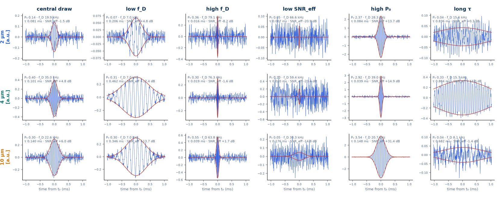
The measured targets the generator reproduces
| Class | n | P₀ · a.u. · median (q05–q95) | f_D · kHz · median (q05–q95) | τ · ms · median (q05–q95) | SNR · dB · median (q05–q95) |
|---|---|---|---|---|---|
| 2 µm | 826 | 0.123 (0.077–0.243) | 16.899 (10.065–34.081) | 0.161 (0.082–0.335) | -0.373 (-6.744–5.205) |
| 4 µm | 1233 | 0.387 (0.208–0.527) | 31.1 (12.413–35.63) | 0.111 (0.087–0.283) | 5.237 (-3.17–12.416) |
| 10 µm | 462 | 0.273 (0.103–0.803) | 18.89 (9.529–27.583) | 0.169 (0.109–0.372) | 6.822 (-0.098–15.032) |
| Class | Row | log P₀ | f_D | log τ | SNR |
|---|---|---|---|---|---|
| 2 µm | log P₀ | 1.00 | · | · | · |
| f_D | 0.30 | 0.95 | · | · | |
| log τ | -0.41 | -0.68 | 0.61 | · | |
| SNR | 0.44 | -0.65 | 0.39 | 0.48 | |
| 4 µm | log P₀ | 1.00 | · | · | · |
| f_D | -0.11 | 0.99 | · | · | |
| log τ | -0.15 | -0.80 | 0.58 | · | |
| SNR | 0.46 | -0.51 | 0.33 | 0.65 | |
| 10 µm | log P₀ | 1.00 | · | · | · |
| f_D | 0.29 | 0.96 | · | · | |
| log τ | -0.37 | -0.72 | 0.58 | · | |
| SNR | 0.79 | -0.44 | 0.22 | 0.37 |
The generator models four coordinates with recorded noise. A fifth asymmetry coordinate was explored and rejected: it improved coverage but not the later learning task.
04 / Learn blind
The model predicts the trace
while it cannot see it.
A real bead record, never used in training. The shaded bands are the 64 hidden windows of 16 samples, 25 % of the trace. The green curve is drawn only where samples were hidden.
Compare it with the simplest honest baseline, a straight line across each gap. The gap between the two is what reconstruction learned about how a passage evolves.
Hidden-window error 0.0016 for the U-Net · 0.0367 for linear interpolation
Did it just memorise the training set?
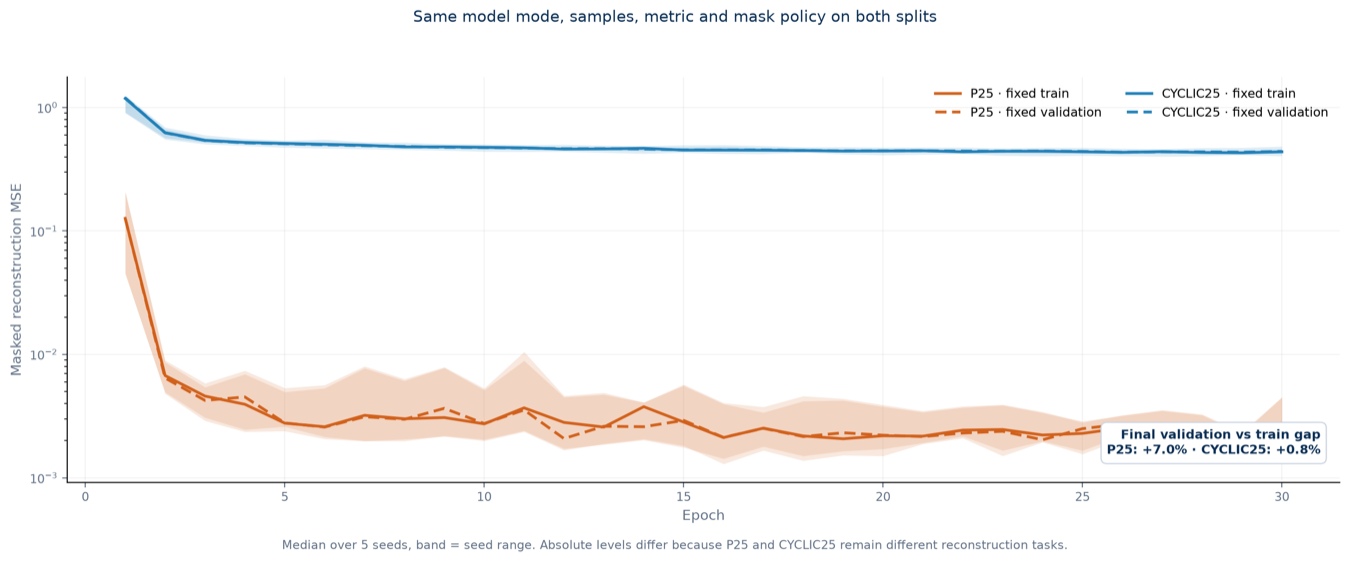
Validation error tracks training error within 1 % under the event-aware mask over 30 epochs (median of five seeds), so the reconstruction task generalises to held-out synthetic records. Against a same-size Transformer trained under identical conditions, the U-Net reduced masked error by about 66 % on both synthetic and real signals; that single-seed comparison selected it.
05 / The reveal
Three groups form
before anyone knows the sizes.
451 real bead passages from recording sources withheld from training pass through the frozen encoder. Their features are scaled, then grouped by k-means into three clusters in the full 96-dimensional space. Only afterwards are the bead sizes revealed to name and score the clusters.
Step through the reveal. Then switch to the supervised reference, a compact classifier trained with the sizes, to see how much of its grouping the label-free encoder recovered.
Hover or select a dot to read that passage’s measured physics.
Exactly what was withheld, and what was not
- Withheld from training: every real event. The encoder saw only synthetic records built from other recordings.
- Withheld from clustering: every label. StandardScaler, row normalisation, PCA and k-means (k = 3, 20 initialisations) are fitted on the 451 events without their sizes.
- Used afterwards: the sizes, to pair each cluster with the size it contains most (Hungarian matching) and to count agreement. Adjusted Rand index: 0.327 for the U-Net, 0.448 for the supervised reference.
- Display only: the two axes are a PCA of the features; the regions are that plane’s section through the 96-dimensional cluster boundaries.
What the features respond to
Frequency and noise are ordered.
Phase is not.
Sweep one physical parameter through 450 synthetic events and watch where they land in the same latent space. A smooth colour gradient means the encoder ordered that parameter.
The self-supervised U-Net orders Doppler frequency and signal-to-noise clearly, amplitude and width weakly, and ignores phase and position: it reads shape, not alignment. The supervised reference orders amplitude and width more sharply.
06 / Towards yeast
A first step.
A bounded claim.
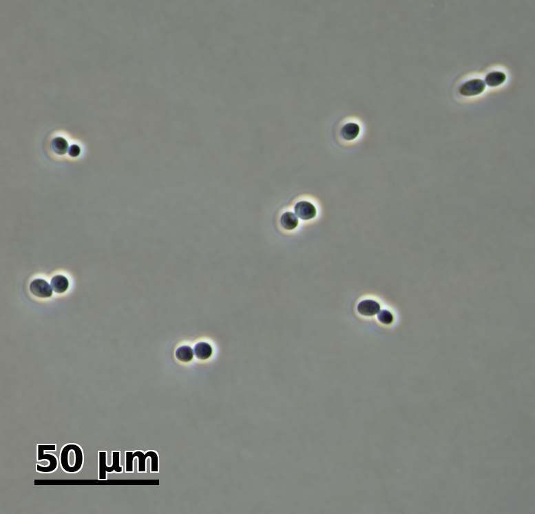
Budding yeast is why this matters. In a single field, budding pairs and isolated cells coexist, and a mother with its bud can produce two delayed responses that split one passage into several Fourier maxima. That is why detection groups energy in time first, and why per-event labels cannot be inherited from the well.
The bead result shows that useful signal structure survives both the synthetic-to-real gap and the absence of labels. What it does not show is listed below.
What the evidence supports
Grouping, not accuracy.
- k-means is fitted and scored on the same 451 events: the percentages describe how those events group, not accuracy on new events.
- One encoder training seed. The three k-means starts test clustering stability only.
- The supervised reference is still sharper overall; the U-Net matches it only on the 4 µm group.
- Synthetic records cover most measured events, not all of them; a real-versus-synthetic classifier can still tell them apart.
- No biological identity is claimed. The next steps are a common labelled task for both encoders, several training seeds, and yeast recordings synchronised with a reference observation of the same cell.
The academic foundations